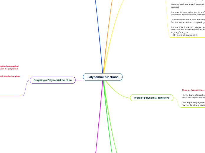
Polynomial functions
Polynomial Expression
A polynomial expression is made up of one or more monomials. There could be a single monomial or multiple separated by operations.
Example: 3x2 + 5x + 2 or 6x
Note:
1) If an exponent is being used, It must be non-negative
Example: 3x4 👍. 5x-2 👎
2) A constant cannot have 2 different variables
Example: 3xy 👎 instead do 3x or 3y 👍.
A monomial can contain
1) A coefficient, this has to be a real number: 3
2) A variable: x
3) A non-negative whole number exponent: ax2
when you put these three together, you have: 3x2
it isn't mandatory for the monomial to contain all three parts. it could be just the constant ( 3 ), the constant with a variable (3x), just the variable (x : keep in mind there's an imaginary 1 at the front) and a variable with an exponent (x3).
Polynomial Function
A polynomial function is when the independent variable is apart of the the polynomial expression
Example:
f(x) = 3x2 + 5x + 2
Criteria for a Polynomial Function
1) The Leading coefficients cannot equal zero and all the following coefficients are all real numbers
2) The exponents are all whole numbers
Things to take note of in a Polynomial Function
- Degrees: The highest exponent monomial in a polynomial represents the degree of the function
Example: In the function: f(x) = 3x2 + 2x + 5 the degree for the function is 2 since thats the highest exponent in the function.
- Leading Coefficient: A coefficient which contains the highest exponent
Examples: In the same function: f(x) = 3x2 + 2x + 5 since 3x2 contains the highest exponent , the leading coefficient is 3.
- If you know an element in the domain of any polynomial function, you can find the corresponding value in the range
Example: If the domain is 3 / f(3), you replace the variable with the value 3. The answer will represent the range.
f(3) = 3(3)2 + 2(3) + 5
= 38 Therefore the range is 38
Types of polynomial functions
There are five main types of polynomials.
- As the degree of the polynomial function increases, the name and various aspects of the function changes.
- The degree of a polynomial function can be more than 4, however the primary focus is going to be up to that point.
Constant:
- has no degree
f(x)= a
f(x) = 5
Linear:
- Has a degree of 1
f(x) = ax + b
f(x) = 4x + 7
Quadratic:
- Has a degree of 2
f(x)= ax2 + bx + c
f(x) = 5x2 + 5x +8
Cubic:
- Has a degree of 3
f(x) = ax3 + bx2 - cx +d
f(x) = 7x3 + 3x2 + 4x + 3
Quartic:
- Has a degree of 4
f(x) = ax4 + bx3 + cx2 + dx + e
f(x) = 3x4 + 2x3 + 7x2 + 3
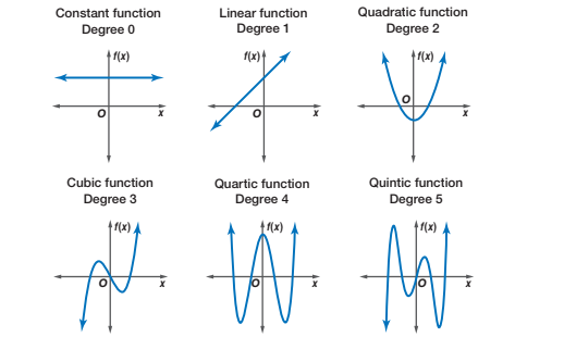
Here's a graphed version of each type of polynomial function:
Finite Differences
It's a tool which helps identify the what type of function the polynomial is.
Step by step on how to use finite difference to find what type of polynomial a polynomial function is.
If it increases at a constant pace during the...
First Difference: It linear
Second Difference: It's Quadratic
Third Difference: It's Cubic
Fourth Difference: It's Quartic
Graphing a Polynomial function
You can guess how a polynomial function looks graphed based on the information given to us in the polynomial function.
1) The amount of arms the polynomial function has when graphed.
2) The amount of roots it have.
3) Turning Points
4) End Behaviours
Number of arms:
The amount of arms a graph has reflects the degree of the function.
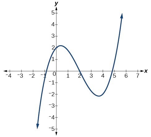
As you can see this graphed polynomial function has three arms. This causes me to believe that it's a cubic function. since a cubic functions have a degree of three.
Roots:
- Roots are the points where the graphed polynomial function intersects the X axis
- at most, a graphed polynomial function has the same amount of roots as the degrees in the function.
Note:
- An even degree polynomial can potentially have no roots since they have similar end behaviours
- For odd functions there must be one root
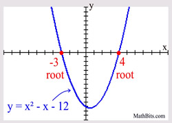
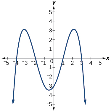
This is a graph of a quadratic function. Just like how a quadratic function has a degree of 2, there are only 2 roots.
End Behaviours:
- End Behaviours focus on which quadrant a graphed polynomial function begins and ends at.
- The factors we use to determine the end behaviours is whether the function has an even or odd degree and whether the leading coefficient is positive or negative.
Even degree function with positive leading coefficient:
Extends from the second quadrant to the first
Even degree function with negative leading coefficient:
Extends from third quadrant to fourth quadrant
Odd degree function with positive leading coefficient:
Extends from third quadrant to first quadrant
Odd degree function with negative leading coefficient
Extends from second quadrant to fourth quadrant
Even functions are symmetric about the Y-axis, while, odd functions have symmetry about the origin.
Turning Points:
- In order to determine the amount of turning points a polynomial function has, you need to subtract 1 from the degree of the function.
Example: 4x3 + 5x2 +7x + 6, Has a degree of 3. when you subtract 3 by 1 you get 2. That means the max amount of turning points this polynomial function will have is 2.
- There are 4 types of turning points: Local max, Local min, Absolute max, Absolute min
- The local max and min are both turning points which are lower than the highest and lowest turning point.
- The Absolute max is the highest turning point while the Absolute min is the lowest turning point. (This is only present in even degree functions)

Factored form
A polynomial function in factored form is used to help find the roots (when the graphed polynomial function intersects the X-axis).
How factored form look like for each type of polynomial function
Quadratic: f(x) = a(x - s)(x - t). x= s,t (this has two roots)
Cubic: f(x) = a(x - s)(x - t)(x - k). x= s,t,k. ( this has three roots)
Quartic: f(x) = a(x - s)(x - t)(x - k)(x- z) x= s,t,k,z (this has four roots)
Perfect Square Quadratic: f(x) = (a - r)2 x= r (this only has one root)
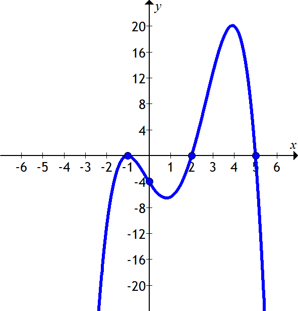
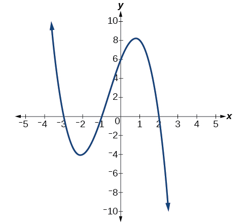
In this graphed relation, the roots are -1, 2 and 5. in factored form it would look like (X + 1) (X -2) (X - 5)
Note: the value in the brackets is the opposite when graphed
Division of Polynomials
There are only two ways to divide Polynomials
1) Synthetic Division
2) Long Division
- Before you do any type of division, it's mandatory to write both the divisor and dividend in descending powers of the variables
Example: 3x2 + 3. ----> 3x2 + 0x + 3 (fill all the missing coefficients with 0.
Synthetic Division:
- It's ideal to use synthetic division when the divisor is (N - 2)
Step by step on how to do Synthetic division:
https://www.wtamu.edu/academic/anns/mps/math/mathlab/col_algebra/col_alg_tut37_syndiv.htm
Long Division
- It's ideal to use long division when the divisor is (N -2)
Step by step on how to do long division
https://www.wtamu.edu/academic/anns/mps/math/mathlab/col_algebra/col_alg_tut36_longdiv.htm
Remainder Theorem and Factor Theorem
Factor Theorem
- Factor theorem is used to determine the factor of a polynomial function without the use of division.
- the divisor is a factor of the dividend only when the remainder equals zero
Step by step on how to use factor theorem
Remainder Theorem:
- Remainder theorem is used to determine the remainder of a divided polynomial without the use of division
Steps by step on how to do remainder theorem